Consider a planet of radius $R_P$ and mass $M_P$ orbitting a star of radius $R_{*}$ and mass $M_{*}$. Let’s define the ratio of planet-to-star radius $k$ as:

The distance between the star and the planet, $r$, is given by:

where $a$ is the semi-major axis and $f$ is the true anomaly, an implicit function of orbital eccentricity $e$ and period $P$ (ie. where the planet is at a given time in its orbit).

We can resolve this into Cartesian coordinate equations within our defined coordinate system.

where $\omega$ represents the argument of periapsis and $i$ represents the inclination.

We can use Pythagorean theorem to derive the projected distance on the sky plane as:

and substituting in equations 3 and 4 for $X$ and $Y$ gives us:

If an eclipse occurs, it will do so at a local minimum of $r_{sky}$. Minimising this expression is long and difficult, but we can approximate by stating that eclipses are centred around conjunctions, which are defined by $X=0$. Conjunctions can either be superior, with the planet in front (a transit); or inferior, with the planet behind (an occultation).

We can find expressions for $f$ for both a transit:

an an occultation:

This approximation is normally valid except for extremely eccentric and close-in orbits, and most importantly for non-grazing orbits. If an orbit is grazing, then a small error can mean the difference between an eclipse and no eclipse.

The impact parameter $b$ is the sky-projected distance at the conjunction, in units of stellar radius:

It ranges $0 \leq b$, where $b = 0$ describes where the planet appears to the observer to pass through the star’s centre; $b = 1$ describes a grazing transit, where the planet passes along the edge of the star; and $b > 1$ represents no eclipse. It is a function of the inclination $i$ and eccentricity of the orbit $e$, and we can derive the two expressions for it below:

We can simplify this further. For the common case where the stellar radius is much smaller than the orbits semi-major axis, $R_{*} « a$, then the exoplanet’s path across the star can be approximated by a straight line between the two points:

Probability of eclipse

Let’s use the above equations to attempt to derive the probability of being able to observe an eclipse by an observer randomly placed on the celestial sphere surrounding the star.

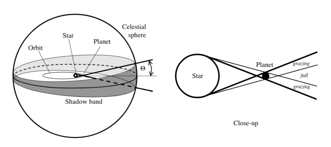
Consider below the excellent figure from the Winn 2010 paper:

Figure 1 shows how an orbiting exoplanet has a shadow cone with angle $\Theta$ which satisfies the conditon:

where $r$ is the actual (non-projected) 3D distance.

The larger cone shown by the thick lines in the right panel of figure 1 is called the penumbra. The penumbra sweeps out a shadow band on the celestial sphere, as seen in the left panel of figure 1. Any observer must be located inside that shadow band in order to observe the eclipse. For them, the impact paramter $b$ will lie in the range $0 \leq b \leq 1$.

The interior cone described by the thinner lines is called the antumbra and satisfies the condition:

Only from within the shadow band swept out by this smaller cone will the eclipse be non-grazing, so the impact parameter $b$ will lie in the range $0 \leq b < 1$.

The Doppler Method for detecting exoplanets can reveal the eccentricity $e$ and argument of periapsis $w$, but the inclination $i$ remains unknown. This works, briefly explained, by taking advantage of the tiny orbit of the star around the system’s centre of mass. This presents as a tiny wobble, where the star’s light will be slightly blueshifted as the star moves towards the observer, and slightly redshifted as it moves away.

Looking at equation 10 and the definiton of the impact parameter $b$, we know that an eclipse occurs where $0 \leq b < 1$ so the condition can be written as $\lvert b \rvert < 1 + k$. We can substitute this into equations 11 and 12, and rearrange to solve for $\cos i$. We know that $0^{\circ} \leq i \leq 90^{\circ}$ which means that $0 \leq \cos i \leq 1$, so:

where the $+$ includes grazing eclipses and the $-$ sign excludes them.

Consider the case where the planet’s radius is significantly smaller than the star’s $R_{P} \ll R_{*}$ and where the orbit is circular $e = 0$:

where $R_{☉}$ represents the radius of the star in terms of solar radius.

This equation tells us a few things. Firstly, for circular orbits, transits and occultations usually occur together. Only highly eccentric orbits allow for a transit or occultation to be observed without the other. Secondly, it frames the transit probability in terms of solar radius and astronomical units. For example, a planet orbiting a Sun-like star at a distance of 1AU has a 0.5% chance of being observable via eclipse from a randomly placed observer. Thirdly, the probability increases in $R_{☉}$ and decreases in $a$. Therefore, the most likely planet’s to be detected are exoplanets with extremely tight orbits around very large stars.

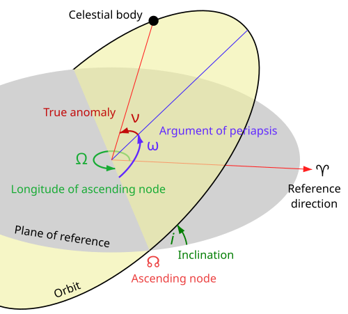
By doing so, we also need to be aware of how the ellipse could be rotated:

• A rotation in the plane of reference affects the longitude of the ascending node $\Omega$ in the diagram below.
• A rotation in the orbital plane affects the argument of periapsis $\omega$ in the diagram below.
• A rotation about the X-axis affects the inclination $i$ in the diagram below.

We are free to define the coordinate system to make our lives as easy as possible. Previously, the orbit was flat on the XY-plane, but now we define the orbit as originally flat on the XZ-plane, or the reference frame.

We also previously defined the origin as the centre of the ellipse, with the star offset on the X-axis by $c$, but now we define the star at the origin with the ellipse offset on the X-axis by $c$.

We place the observer at (0, 0, large positive Z).

Line of nodes and Longitude of the ascending node

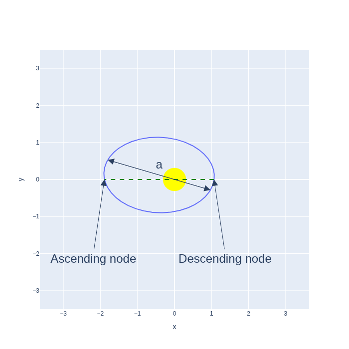
Consider below an orthographic projection for the view of the elliptical orbit from the observer’s perspective. We could also call this projection the sky-plane, as seen on the celestial sphere about the observer.

Where the orbiting object crosses $z=0$ moving towards the observer, so into positive $z$, is called the descending node. Where the orbiting object crosses $z=0$ moving away from the observer, so into negative $z$, is called the ascending node.

A straight line connecting these two, passing through the centre of the star, is called the line of nodes, as shown by the green dashed line in Figure 2.

Since the longitude of the ascending node drawn on the celestial sphere is usually difficult to actually know, and is often entirely unknown, we simply define the X-axis to align with this line, so that the descending node is in positive $x$ and the ascending node is in negative $x$. This results in $\Omega = 180^{\circ}$ and removes the concept of rotation about the Z-axis entirely, simplifying our maths.

Argument of Periapsis

Figure 2 does, however, show the ellipse rotated in the orbital plane. The angle of rotation is called the argument of periapsis $\omega$.

The line below labeled $a$ shows the semi-major axis, connecting the periapsis and apoapsis of the elliptical orbit. In our 2d diagrams, we defined the X-axis as being aligned with the semi-major axis, so this rotation was irrelevant. However, since we define the X-axis as aligning with the line of nodes, this rotation becomes relevant and explains why the line of nodes does not necessarily always align with the semi-major axis.

The argument of periapsis is not labelled in Figure 2, because the diagram shows the orbit on the sky plane, but the rotation is applied in the orbital plane. See Figure 1 for labelled $\omega$.

Inclination

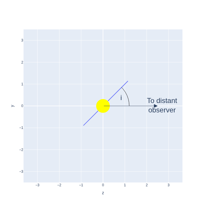
The value of the inclination represents how much the orbit is rotated about the Y-axis. The inclination is measured in radians within the range $0 \leq i \leq \pi$, where $i = 0$ represents an orbit flat on the reference frame and $i = \pi$ represents an orbit orthogonal to the reference frame.

3D model

To recap our coordinate system: we define the star at the origin, with ourselves, the observer, at large positive Z. To simplify the maths, we define the X-axis to be aligned with the line of nodes. The Y-axis is then the only possible remaining direction which is orthogonal to both the Z- and X-axes.

The 3D model below shows a distant observer, a star (the yellow sphere) and an elliptical orbit around it (blue curve). The blue plane is the XY, or sky, plane, as viewed from the observer, centred around the star. The orange plane is the orbital plane.

Explore the 3D model by panning and zooming to ensure you understand the geometry of elliptical orbits in three dimensions.

Technical definiton of ellipse: for any point on the ellipse, the sum of distances to each focus is constant.

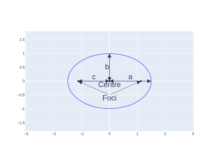
See labelled diagram for an ellipse below for the names of the different components.

• Semi-major axis, $a$
• Semi-minor axis, $b$
• Distance from centre to focus, $c$

The distance from centre to focus, $c$ is geometrically related to the semi-major and -minor axes by the equation:

Here we can define a new term - the eccentricty $e$ - which is related to $c$ and $a$ by:

When $e=0$, then the ellipse is a special case - a circle. Ellipses have eccentricities $0 \leq e < 1$. Where $e=1$, the ellipse is now unbound and becomes a parabola, and where $e>1$ the eccentricity is so extreme that we refer to the curve as a hyperbola.

Elliptical orbits

Planet’s have elliptical orbits around their star, which is found at one of the focus points. Technically, both the star and planet have elliptical orbits around the system’s centre of mass, which is found at the shared focus of every elliptical orbit of each object in the system. Understanding this is important for understanding other methods for detecting exoplanets, such as the Doppler Method. But for our purposes, the star’s mass is usually so much greater than the plantary mass, and the star’s orbit so much smaller in comparison to the planet’s orbit, that it is helpful for us to simplify and imagine that the star is fixed at the focus point of a planet’s elliptical orbit around it.

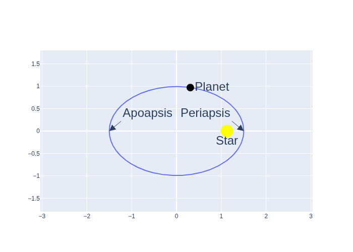
The point on the orbit where the planet is closest to its star is called the periapsis, or when the star is the Sun, it is called the perihelion. The opposite point, where it is furthest from its star, is called the apoapsis, or when the star is the Sun, it is called the aphelion.

Anomalies and Kepler’s Second Law

Kepler’s Second Law states that a line from an object on an elliptical orbit to the star at one of its focal points will sweep out equal areas during equal intervals in time. This basically means that an object moves faster when its closer to its star and slower when its further away.

In order to accurately animate orbital motion with Kepler’s Second Law, we must understand elliptical anomalies.

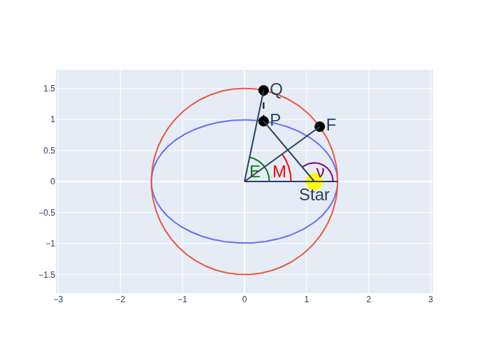
Imagine a circle with radius $a$ centred at the origin.

Mean Anomaly

Consider a hypothetical planet completing a full orbit in the same time period $T$ as our real planet on its elliptical orbit.

This hypothetical planet has constant angular speed, described by:

The mean anomaly $M$ is the angle from the origin between the periapsis and the point $F$ on the imaginary orbit for given $t$, when $t=0$ at the periapsis.

Eccentric Anomaly

Take the point $P$ on the ellipitcal orbit, where the planet actually is at time $t$, and project upwards to the imaginary circle at point $Q$.

The eccentric anomaly $E$ is the angle from the origin between the periapsis and point $Q$.

True Anomaly

True anomaly $\nu$ is simply the angle from the star between the periapsis and the planet’s real position on the ellipitcal orbit at time $t$.

Computing eccentric anomaly from mean anomaly

Kepler found the below equation linking the mean and eccentric anomaly:

So to animate our elliptical orbit with Kepler’s Second Law, we can solve for $E(t)$ to find where the planet should be on the hypotehtical circle, then project straight down until we meet the ellipse.

However, there is a problem. The above formula cannot be solved for $E$ in closed form. Enter: Newton’s iterative method for finding the root of an equation.

We can rewrite the above equation to

which turns the problem into a root finding problem - we can find $E$ from $M$ where $f(E) = 0$.

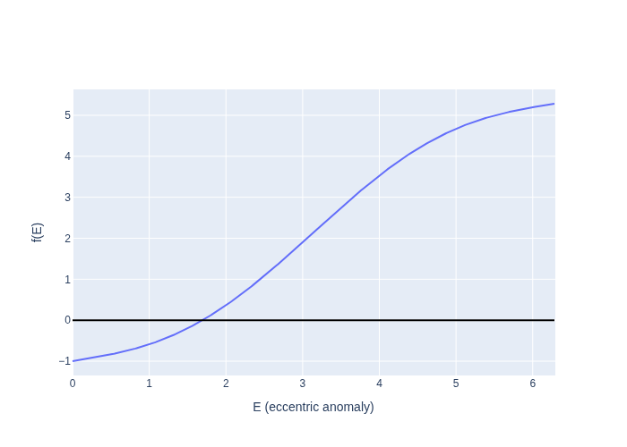
Let’s visualise this equation graphically. We can graph $f(E)$ for given values of $e$ and $M$. Here, $e = 0.7$ and $M=3$:

Then we take an initial guess. For us, a reasonable first guess is $E_0 = M$. Using the below equation, we can refine our guess to find the value of $E$ where $f(E) = 0$:

Let’s understand what we’re doing here. The numerator, $f(E_n)$, tells us whether we’re above or below the root, and by how far. The denominator tells us the gradient of the curve at this value of $E$. Looking at the curve, we know the gradient will be shallow far from the root and steep close to the root. When the gradient is shallow, the denominator will be small, so the step from $E_n$ to $E_{n+1}$ will be large, and vice versa when the gradient is steep.

We can substitute $f(E) = E - e \sin E - M$ and $f’(E) = 1 - e \cos E$ (knowing that the first derivative of $e \sin E$ is $e \cos E$) to write the equation in terms that we can calculate:

For our purposes, only 5 iterations of the above formula will give a value of $E$ so that $f(E)$ is extremely close to $0$.

We can then derive cartesian coordinates of the elliptical orbit using the below equations:

And drawing these coordinates in discrete time intervals gives the below animation, showing Kepler’s Second Law in action.

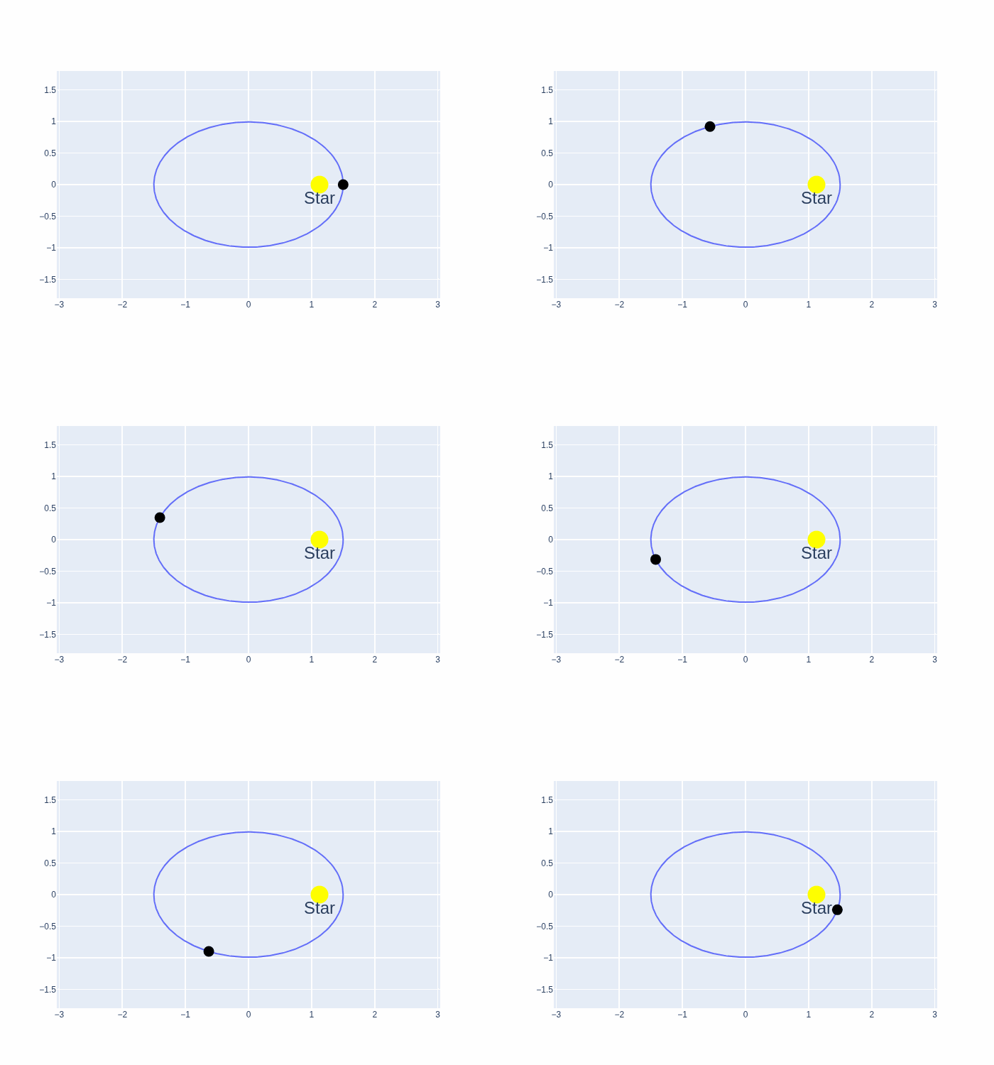
The object has an elliptical orbit around the star, moving quickly near the periapsis and slowly near the apoapsis.