Eclipse Basics
Geometry of eclipses
Consider a planet of radius $R_P$ and mass $M_P$ orbitting a star of radius $R_{*}$ and mass $M_{*}$. Let’s define the ratio of planet-to-star radius $k$ as:
\[k = \frac{R_P}{R_*} \tag{1}\]The distance between the star and the planet, $r$, is given by:
\[r = \frac{a(1 - e^2)}{1 + e \cos f} \tag{2}\]where $a$ is the semi-major axis and $f$ is the true anomaly, an implicit function of orbital eccentricity $e$ and period $P$ (ie. where the planet is at a given time in its orbit).
We can resolve this into Cartesian coordinate equations within our defined coordinate system.
\[X = -r \cos (\omega + f) \tag{3}\] \[Y = -r \sin (\omega + f) \cos i \tag{4}\] \[Z = r \sin (\omega + f) \sin i \tag{5}\]where $\omega$ represents the argument of periapsis and $i$ represents the inclination.
We can use Pythagorean theorem to derive the projected distance on the sky plane as:
\[r_{sky} \equiv \sqrt{X^2 + Y^2} \tag{6}\]and substituting in equations 3 and 4 for $X$ and $Y$ gives us:
\[r_{sky} = \frac{a(1-e^2)}{1 + e \cos f} \sqrt{1 - \sin ^2 {(\omega + f)} \sin^2 {i}} \tag{7}\]If an eclipse occurs, it will do so at a local minimum of $r_{sky}$. Minimising this expression is long and difficult, but we can approximate by stating that eclipses are centred around conjunctions, which are defined by $X=0$. Conjunctions can either be superior, with the planet in front (a transit); or inferior, with the planet behind (an occultation).
We can find expressions for $f$ for both a transit:
\[f_{tra} = + \frac{\pi}{2} - w \tag{8}\]an an occultation:
\[f_{occ} = - \frac{\pi}{2} - w \tag{9}\]This approximation is normally valid except for extremely eccentric and close-in orbits, and most importantly for non-grazing orbits. If an orbit is grazing, then a small error can mean the difference between an eclipse and no eclipse.
The impact parameter $b$ is the sky-projected distance at the conjunction, in units of stellar radius:
\[b \equiv \frac{r_{sky}}{R_{*}} = \frac{R_{*} + R_{P}}{R{*}} = 1 + k \tag{10}\]It ranges $0 \leq b$, where $b = 0$ describes where the planet appears to the observer to pass through the star’s centre; $b = 1$ describes a grazing transit, where the planet passes along the edge of the star; and $b > 1$ represents no eclipse. It is a function of the inclination $i$ and eccentricity of the orbit $e$, and we can derive the two expressions for it below:
\[b_{tra} = \frac{a \cos i}{R_{*}} \left( \frac{1 - e^2}{1 + e \sin \omega} \right) \tag{11}\] \[b_{occ} = \frac{a \cos i}{R_{*}} \left( \frac{1 - e^2}{1 - e \sin \omega} \right) \tag{12}\]We can simplify this further. For the common case where the stellar radius is much smaller than the orbits semi-major axis, $R_{*} « a$, then the exoplanet’s path across the star can be approximated by a straight line between the two points:
\[X = \pm R_{*} \sqrt{1 - b^2} \tag{13}\]Probability of eclipse
Let’s use the above equations to attempt to derive the probability of being able to observe an eclipse by an observer randomly placed on the celestial sphere surrounding the star.
Consider below the excellent figure from the Winn 2010 paper:
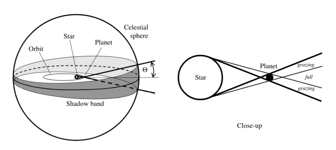
Figure 1 shows how an orbiting exoplanet has a shadow cone with angle $\Theta$ which satisfies the conditon:
\[\sin \Theta = \frac{R_{*} + R_p}{r} \tag{14}\]where $r$ is the actual (non-projected) 3D distance.
The larger cone shown by the thick lines in the right panel of figure 1 is called the penumbra. The penumbra sweeps out a shadow band on the celestial sphere, as seen in the left panel of figure 1. Any observer must be located inside that shadow band in order to observe the eclipse. For them, the impact paramter $b$ will lie in the range $0 \leq b \leq 1$.
The interior cone described by the thinner lines is called the antumbra and satisfies the condition:
\[\sin \Theta = \frac{R_{*} - R_p}{r} \tag{15}\]Only from within the shadow band swept out by this smaller cone will the eclipse be non-grazing, so the impact parameter $b$ will lie in the range $0 \leq b < 1$.
The Doppler Method for detecting exoplanets can reveal the eccentricity $e$ and argument of periapsis $w$, but the inclination $i$ remains unknown. This works, briefly explained, by taking advantage of the tiny orbit of the star around the system’s centre of mass. This presents as a tiny wobble, where the star’s light will be slightly blueshifted as the star moves towards the observer, and slightly redshifted as it moves away.
Looking at equation 10 and the definiton of the impact parameter $b$, we know that an eclipse occurs where $0 \leq b < 1$ so the condition can be written as $\lvert b \rvert < 1 + k$. We can substitute this into equations 11 and 12, and rearrange to solve for $\cos i$. We know that $0^{\circ} \leq i \leq 90^{\circ}$ which means that $0 \leq \cos i \leq 1$, so:
\[p_{tra} = \left( \frac{R_{*} \pm R_{P}}{a} \right) \left( \frac{1 + e \sin \omega}{1 - e^2} \right) \tag{16}\] \[p_{occ} = \left( \frac{R_{*} \pm R_{P}}{a} \right) \left( \frac{1 - e \sin \omega}{1 - e^2} \right) \tag{17}\]where the $+$ includes grazing eclipses and the $-$ sign excludes them.
Consider the case where the planet’s radius is significantly smaller than the star’s $R_{P} \ll R_{*}$ and where the orbit is circular $e = 0$:
\[p_{tra} = p_{occ} = \frac{R_{*}}{a} \approx 0.0005 \left( \frac{R_{*}}{R_{☉}} \right) \left( \frac{a}{1 AU} \right) ^{-1} \tag{18}\]where $R_{☉}$ represents the radius of the star in terms of solar radius.
This equation tells us a few things. Firstly, for circular orbits, transits and occultations usually occur together. Only highly eccentric orbits allow for a transit or occultation to be observed without the other. Secondly, it frames the transit probability in terms of solar radius and astronomical units. For example, a planet orbiting a Sun-like star at a distance of 1AU has a 0.5% chance of being observable via eclipse from a randomly placed observer. Thirdly, the probability increases in $R_{☉}$ and decreases in $a$. Therefore, the most likely planet’s to be detected are exoplanets with extremely tight orbits around very large stars.